If you live in a big city, wasting your life away in traffic is probably just another part of your daily life. Planning ahead your commutes can help you save some time but it’s not that always that simple. Learning the road traffic patterns in your city may come with experience but you can not always rely on that.
Unlike cars on the road, the more data we have, the better our commute planning can be.
Uber Movement Speed Dataset
Uber recently released their Uber Movement Street Speeds for five cities: New York City, Seattle, Cincinnati, Nairobi and London. For this post we will explore the New York City dataset. The dataset consists of a the main data in csv form broken down by month per file. There are also metadata CSV files for hourly statistics and OpenStreetMaps node ID’s.
Exploring the data
Raw data – as with the food are rarely digestibe as is. The speed movement data is not the exception here. Uber’s suggestion was to begin exploration with their open source geospacial visualzation app – kepler.gl
By cross-referencing Uber’s data to OpenStreetMap we could get the coordinates of the road segment to use in our plotting and data analysis. I’ve uploaded an instance of kepler.gl loaded with the uber data that you can view here. The website is quite resource intensive though so if you’re reading from a phone, you might want to wait until you’re on your more powerful computer before you start exploring the visualzation.
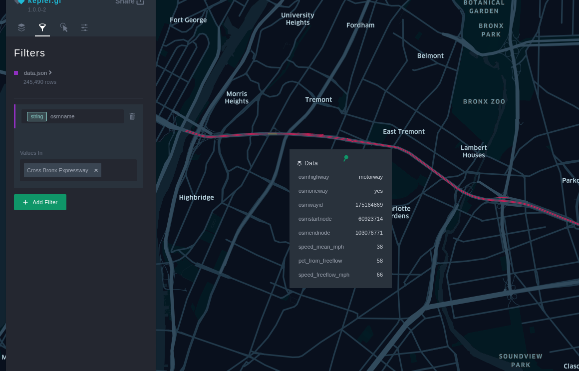
Exploring Cross Bronx Expressway segment data Kepler
Travel Time Calculation
Given the speed data on the road segments, it should be possible to calculate travel time given any paths on the road and the time. One challenge though is to figure out which road segments to use on the calculation. First we need to fine a set of points that will serve will draw a path from a beginning location to the destination. For that task, we can use openrouteservice.org to generate the geocoordinates from text address and to provide as a set of path points for navigation.
import openrouteservice
from_loc = 'Empire State Building, New York'
to_loc = 'Central Park, Manhattan'
client = openrouteservice.Client(key=api_key)

empire_state = client.pelias_search(
    from_loc)['features'][0]['geometry']['coordinates']
central_park = client.pelias_search(
    to_loc)['features'][0]['geometry']['coordinates']

coords = (empire_state, central_park)
routes = client.directions(coords)Finally, we need to address the issue with road segments pointing the opposite direction. Luckily the starting point and the ending point for each road segments are labeled so we can use that to determine the flow of traffic on that road segment. I used the atan2 function to get a numeric representation of the direction that we can easily compare between a pair of path points and the nearby line segments.
So now that we’re done with filtering, we need to calculate the distance travelled so we can divide it by our movement speed to get the travel time. To this with decent accuracy, I used the geodesic distance between the points of the line segments. The resulting distance is then divided by the average speed of the road segment with the most overlap with the path segment.
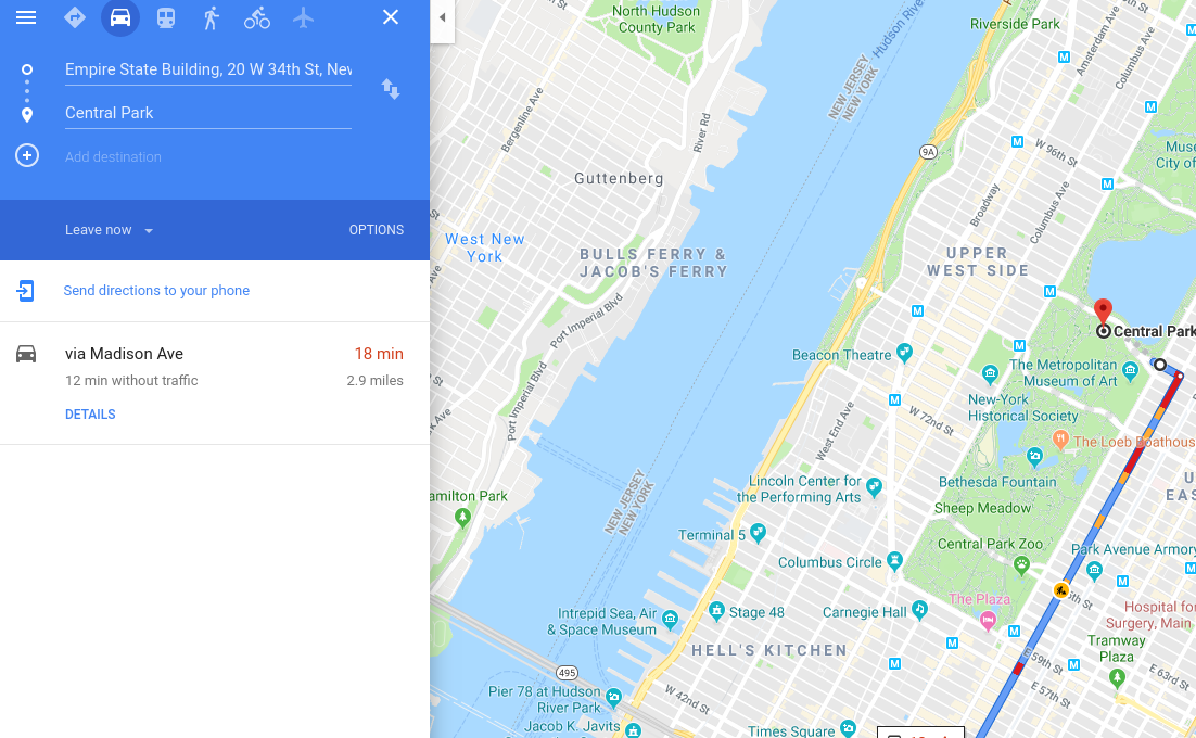
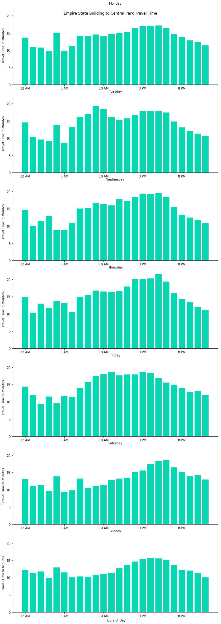
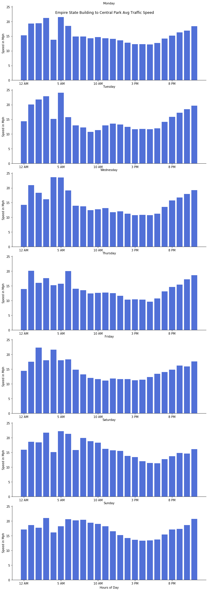
Now that we’ve defined the process, we can now compute the average travel times between any number of places in New York City at any given time (1 hour interval) Here’s what I got from the example above (Empire State Building to Central Park):
Now here’s Google’s computation on the same route for reference: